Sixth Summer School on Computer Vision, Graphics and Image Processing
Machine Learning Algorithms - Hands-on Session 1
Avisek Gupta (avisek003@gmail.com)
Electronics and Communication Sciences Unit
May 31, 2019
Supervised Learning
-
Given: Labeled data
-
Task: Learn to correctly label the given data
-
Objective: Correctly label ANY given data
Unsupervised Learning
-
Given: Data (No labels!)
-
Tasks:
-
Clustering: Find 'similar groups' in the given data
-
Dimension Reduction: Retain 'useful' feature; Discard less useful features
-
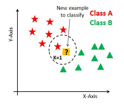
Supervised Learning : $k$-Nearest Neighbours ($k$NN) Classifier
-
Learning Phase: $k$NN 'learns' by simply holding on to the entire dataset
-
How well does $k$NN classify unseen data? Testing Phase: Given an unseen data point $x$, $k$NN finds the $k$ nearest training data points (neighbours) of $x$
Unsupervised Learning : $k$-Means Clustering
-
Randomly select $k$ data points as 'initial' centers
-
Repeat till convergence:
-
Calculate distance of all data points to the $k$ centers
-
Update Cluster Membership: Assign data points to its closest center
-
Update Centers: Calculate the mean of all data points in a cluster
-

-- Numpy Recap --
In [1]:
import numpy as np
1. Array Creation:
In [2]:
A = np.zeros((2, 3)) # Zero-filled array of shape (#rows, #cols)

print('A = \n', A, '\n')

B = np.ones((3, 2)) # One-filled array of shape (#rows, #cols)

print('B = \n', B, '\n')

C = np.array([1,2,3])

print('C = \n', C)
2. Basic Operations: + , - , * , / , @
In [3]:
print('A + 2 =\n', A + 2, '\n')

print('A - C =\n', A - C, '\n')

print('B * 4 =\n', B * 4, '\n')

print('C / 2 =\n', C / 2, '\n')

print('C ** 0.5 =\n', C ** 0.5, '\n')

print('(A + 2) @ B = \n', (A + 2) @ B)
In [4]:
D = np.array([[1, 2], [3, 4], [5, 6]])

print('D =', D, '\n')

print('np.sum(D) =', np.sum(D), '\n')

print('np.sum(D, axis=0) =', np.sum(D, axis=0), '\n')

print('np.sum(D, axis=1) =', np.sum(D, axis=1), '\n')

print('np.mean(D, axis=0) =', np.mean(D, axis=0), '\n')

print('np.var(D, axis=0) =', np.var(D, axis=0), '\n')

print('np.min(D, axis=0) =', np.min(D, axis=0), '\n')

print('np.argmin(D, axis=0) =', np.argmin(D, axis=0), '\n')

print('np.max(D, axis=1) =', np.max(D, axis=1), '\n')

print('np.argmax(D, axis=1) =', np.argmax(D, axis=1), '\n')
3. Get Array Information
In [5]:
print('#dims of A =', A.ndim, '\n')

print('#dims of C =', C.ndim, '\n')

# ~~~~~~~~~~~~~~~~~~~~~~~~~~~ #

print('Shape of A =', A.shape, '\n')

print('Shape of C =', C.shape, '\n')

# ~~~~~~~~~~~~~~~~~~~~~~~~~~~ #

print('Data Type of A =', A.dtype, '\n')
4. Create Random Array
In [6]:
RandX = np.random.rand(2,3)

print('RandX =\n', RandX, '\n')

RandIntX = np.random.randint(0, 10, (2,3))

print('RandIntX =\n', RandIntX, '\n')
5. Reshape an Array
In [7]:
print('RandX =\n', RandX, '\n')

print('RandX.shape =', RandX.shape, '\n')

print('np.reshape(RandX, (3,2)) =\n', np.reshape(RandX, (3,2)), '\n')

print('np.reshape(RandX, (1,6)) =\n', np.reshape(RandX, (1,6)), '\n')
6. Stack Arrays together
In [8]:
print('RandX =\n', RandX, '\n')

print('A =\n', A, '\n')

print('np.vstack((RandX, A)) =\n', np.vstack((RandX, A)), '\n')

print('np.hstack((RandX, A)) =\n', np.hstack((RandX, A)), '\n')
7. Array Indexing
In [9]:
print('RandX =\n', RandX, '\n')

print('RandX[0,1] =\n', RandX[0,1], '\n')

print('RandX[1,:] =\n', RandX[1,:], '\n')

print('RandX[:,2] =\n', RandX[:,2], '\n')

print('RandX[:,-1] =\n', RandX[:,-1], '\n')
8. Boolean Array Indexing
In [10]:
F = np.array([[6, 4], [2, 3], [7, 9]])

print('F =\n', F, '\n')

print('(F==2) =\n', F==2, '\n')

print('(F==np.min(F)) =\n', F==np.min(F), '\n')

print('(F[F==np.min(F)]) =\n', F[F==np.min(F)], '\n')

indices = np.array([True, False, True])

print('indices =\n', indices, '\n')

print('F[indices] =\n', F[indices, :], '\n')
9. Deep Copy vs Shallow Copy
In [11]:
G = F
G[0,0] = 10

print('F =\n', F, '\n')
print('G =\n', G, '\n')


H = np.array(F)
H[0,0] = 2

print('F =\n', F, '\n')
print('H =\n', H, '\n')
-- Matplotlib Recap --
In [12]:
import matplotlib.pyplot as plt
1. A Simple Plot
In [13]:
X = np.array([1,2,3,4,5,6])

Y = X ** 2

plt.figure()

plt.plot(X, Y, c='g')

plt.show()

2. A Simple Scatter Plot
In [14]:
X1 = np.array([[-0.1, 0.1], [-0.2,-0.1], [-0.15, 0.2], [-0.05, -0.05], [0.1,0.1]])
X2 = np.array([[0.2, 0.1], [0.1,0], [0.15, 0.05], [-0.1, -0.2], [0.15,-0.15]])

plt.figure()

plt.scatter(X1[:,0], X1[:,1], c='b', marker='+')
plt.scatter(X2[:,0], X2[:,1], c='r', marker=1)

plt.show()

3. Scatter Plot of 2D Gaussians
In [15]:
X1 = np.random.normal(loc=[0,0], scale=1, size=(50,2))
X2 = np.random.normal(loc=[10,0], scale=1, size=(50,2))

plt.figure(dpi=120)

plt.scatter(X1[:,0], X1[:,1], c='b', marker='x')
plt.scatter(X2[:,0], X2[:,1], c='r', marker='x')

plt.axis('equal')

plt.xlabel('X1', fontsize=12)
plt.ylabel('X2', fontsize=12)
plt.title('X2 vs X1', fontsize=14)

plt.show()

Implementing the $k$NN Classifier
1. Load a data set, divide it into train and test sets
In [16]:
from sklearn.datasets import load_iris
from sklearn.model_selection import train_test_split

X, y = load_iris().data[:,0:2], load_iris().target
X_train, X_test, y_train, y_test = train_test_split(X, y, test_size=0.2)

print(X_train.shape, y_train.shape)
In [17]:
plt.figure(dpi=120)
for i in range(3):
    plt.scatter(X_train[y_train==i,0], X_train[y_train==i,1], marker='x')
plt.show()

2. Select a test point
In [27]:
test_p = X_test[5,:]

plt.figure(dpi=120)
for i in range(3):
    plt.scatter(X_train[y_train==i,0], X_train[y_train==i,1], marker='x')
plt.scatter(test_p[0], test_p[1], marker='o', c='w', edgecolor='k')
plt.show()

3.(i) Calculate the distance of all training points to the test point
(ii) Find the $k$ nearest training points
In [28]:
k = 5


# Calculate distance of test point to all training points
distances = np.zeros((120))
for i in range(120):
    for j in range(2):
        distances[i] += ((X_train[i,j] - test_p[j]) ** 2)

# Find the k nearest training points
knn = np.argsort(distances)[0:k]


plt.figure(dpi=120)
plt.scatter(X_train[knn,0], X_train[knn,1], marker='o', c='w', edgecolor='r', s=80)
for i in range(3):
    plt.scatter(X_train[y_train==i,0], X_train[y_train==i,1], marker='x')
plt.scatter(test_p[0], test_p[1], marker='o', c='w', edgecolor='k')
plt.show()

4. Get the mode of the neighbour labels
In [29]:
from scipy.stats import mode


# Get mode of the labels
y_pred = mode(y_train[knn]).mode[0]


plt.figure(dpi=120)
c = ['C0', 'C1', 'C2']
plt.scatter(X_train[knn,0], X_train[knn,1], marker='o', c='w', edgecolor='r', s=80)
plt.scatter(test_p[0], test_p[1], marker='o', c='w', edgecolor='k', s=80)
for i in range(3):
    plt.scatter(X_train[y_train==i,0], X_train[y_train==i,1], marker='x')
plt.scatter(test_p[0], test_p[1], marker='x', c=c[y_pred], s=120)
plt.show()

Putting it all together:
In [31]:
import numpy as np
from scipy.stats import mode

def knn_classifier(X_train, ytrain, X_test, k=3):
    # Calculate distance of test point to all training points
    distances = np.sum((X_train - X_test) ** 2, axis=1)

    # Find the k nearest training points
    knn = np.argsort(distances)[0:k]

    # Get mode of labels
    y_pred = mode(y_train[knn]).mode[0]

    return y_pred, knn


if __name__ == '__main__':
    from sklearn.datasets import load_iris
    X, y = load_iris().data[:,0:2], load_iris().target
    from sklearn.model_selection import train_test_split
    X_train, X_test, y_train, y_test = train_test_split(X, y, test_size=0.2)

    k = 5
    test_pt = X_test[5,:]
    y_pred, knn = knn_classifier(X_train, y_train, test_pt, k=k)

    import matplotlib.pyplot as plt
    plt.figure(dpi=120)
    c = ['C0', 'C1', 'C2']
    plt.scatter(X_train[knn,0], X_train[knn,1], marker='o', c='w', edgecolor='r', s=80)
    plt.scatter(test_pt[0], test_pt[1], marker='o', c='w', edgecolor='k', s=80)
    for i in range(3):
        plt.scatter(X_train[y_train==i,0], X_train[y_train==i,1], marker='x')
    plt.scatter(test_pt[0], test_pt[1], marker='x', c=c[y_pred], s=120)
    plt.show()

Implementing $k$-Means Clustering
In [22]:
from sklearn.datasets import load_iris

X, y = load_iris().data[:,2:], load_iris().target

print(X.shape, y.shape)
In [23]:
plt.figure(dpi=120)
for i in range(3):
    plt.scatter(X[y==i,0], X[y==i,1], marker='x')
plt.show()

1. Randomly select $k$ cluster centers
In [24]:
k = 3

idx = np.random.permutation(X.shape[0])[0:k]

centers = X[idx, :]


plt.figure(dpi=120)
plt.scatter(centers[:,0], centers[:,1], marker='o', c='w', edgecolor='r', s=80)
plt.scatter(X[:,0], X[:,1], marker='x', c='k')
plt.show()

2. Loop till convergence:
- (i) Calculate distance of all points to the $k$ cluster centers
- (ii) Update Cluster Membership: Assign data points to its closest center
- (iii) Update Centers: Calculate the mean of all data points in a cluster
In [25]:
max_iter = 100


for v_iter in range(max_iter):

    distances = np.zeros((X.shape[0], k))
    for i1 in range(X.shape[0]):
        for i2 in range(k):
            for i3 in range(X.shape[1]):
                distances[i1, i2] += ((X[i1,i3] - centers[i2,i3]) ** 2)

    memberships = np.argmin(distances, axis=1)

    prev_centers = np.array(centers)
    centers = np.zeros((k, X.shape[1]))
    for i1 in range(k):
        count = 0
        for i2 in range(X.shape[0]):
            if memberships[i2] == i1:
                for i3 in range(X.shape[1]):
                    centers[i1,i3] += X[i2,i3]
                count += 1
        for i3 in range(X.shape[1]):
            centers[i1,i3] /= count


plt.figure(dpi=120)
for i in range(k):
    plt.scatter(X[memberships==i,0], X[memberships==i,1], marker='x')
plt.scatter(centers[:,0], centers[:,1], marker='o', c='r')
plt.show()

Putting it all together:
In [26]:
import numpy as np
from scipy.spatial.distance import cdist


def kmeans(X, k, max_iter=300):
    centers = X[np.random.permutation(X.shape[0])[0:k],:]

    for v_iter in range(max_iter):
        distances = cdist(X, centers)

        memberships = np.argmin(distances, axis=1)

        prev_centers = np.array(centers)
        for i in range(k):
            centers[i,:] = np.mean(X[memberships==i], axis=0)

    return centers, memberships


if __name__ == '__main__':
    centers, memberships = kmeans(X, k=3)

    plt.figure(dpi=120)
    for i in range(k):
        plt.scatter(X[memberships==i,0], X[memberships==i,1], marker='x')
    plt.scatter(centers[:,0], centers[:,1], marker='o', c='r')
    plt.show()
