Sixth Summer School on Computer Vision, Graphics and Image Processing
Machine Learning Algorithms Session 2 (b)
Avisek Gupta (avisek003@gmail.com)
Electronics and Communication Sciences Unit
June 04, 2019
Supervised Learning
-
Classification: Learn to predict a class / category
-
Regression: Learn to predict a target real value
Linear Regression:
Find the line that best fits the given data
In [2]:
import numpy as np
import matplotlib.pyplot as plt


data = np.array([
    [0.20, 0.30], [0.32, 0.23], [0.39, 0.35], [0.46, 0.42],
    [0.51, 0.39], [0.60, 0.47], [0.64, 0.51], [0.75, 0.46]
])


plt.figure()
plt.scatter(data[:,0], data[:,1], marker='o', c='C0')
plt.plot([0.1, 0.9], [0.174251 + 0.1*0.448577, 0.174251 + 0.9*0.448577], c='C1', linestyle=':', linewidth=1)
plt.show()

Linear Regression:
1. Regression Model: A straight line $y = w_0 + w_1 x $ .
2. Learning: Given a regression model, estimate the parameters ($w_0, w_1$) of the model.
3. Cost Function:
-
Measures how "bad" the model is.
-
Used to guide the selection of better model parameters.
Measures how "bad" the model is.
Used to guide the selection of better model parameters.
Example of a Cost Function:
Mean Squared Error (MSE) = $\frac{1}{n} \sum_{i=1}^{n} (y_i - (w_0 + w_1 x_i))^2$
In [3]:
import numpy as np
import matplotlib.pyplot as plt


data = np.array([
    [0.20, 0.30], [0.32, 0.23], [0.39, 0.35], [0.46, 0.42],
    [0.51, 0.39], [0.60, 0.47], [0.64, 0.51], [0.75, 0.46]
])
x = data[:,0]
y = data[:,1]


random_w = np.random.rand(2)

mse = np.mean((y - (random_w[0] + random_w[1] * x)) ** 2)
print('MSE =', mse)


plt.figure()
plt.scatter(data[:,0], data[:,1], marker='o', c='C0')
plt.plot([0.1, 0.9], [random_w[0] + 0.1*random_w[1], random_w[0] + 0.9*random_w[1]], c='C1')
plt.show()

Linear Regression:
1. Regression Model: A straight line $y = w_0 + w_1 x $ .
2. Learning: Given a regression model, estimate the parameters ($w_0, w_1$) of the model.
3. Cost Function:
-
Measures how "bad" the model is.
-
Used to guide the selection of better model parameters.
4. Optimization Algorithm:
-
Estimates the model parameters by trying to reduce the cost function.
-
There can be many possible ways to optimize the same cost function.
Measures how "bad" the model is.
Used to guide the selection of better model parameters.
Estimates the model parameters by trying to reduce the cost function.
There can be many possible ways to optimize the same cost function.
Example of an Optimization Algorithm: Gradient Descent
Gradient Descent to optimize a function $f(w)$:
1. Pick a random initital point $w_0$
2. Loop till convergence: $w_{i+1} := w_{i} - \alpha \nabla f(w_{i})$
($\alpha$: Step size)
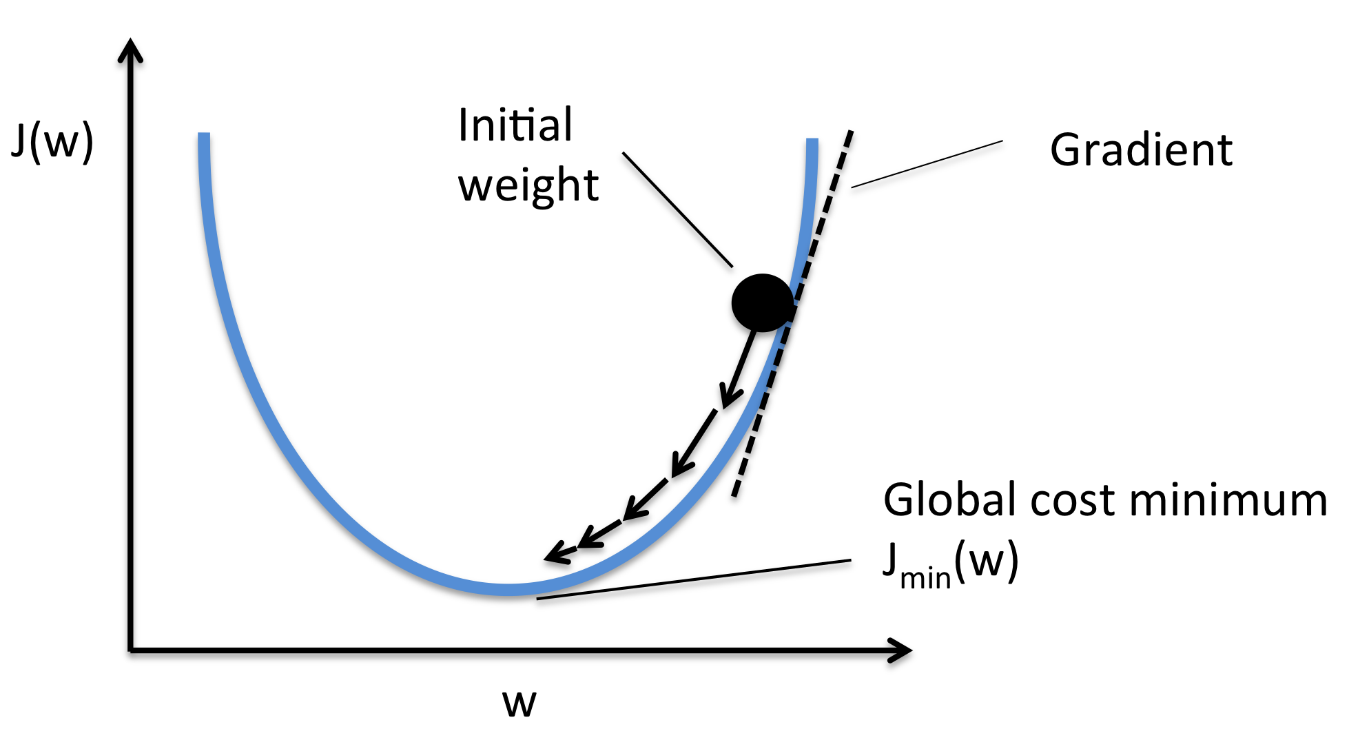
Source: https://rasbt.github.io/mlxtend/user_guide/general_concepts/gradient-optimization/
Example: Gradient Descent of a simple function $f(w) = w^2+4$
Conjugate Gradient Descent: Automatically selects an appropriate step size
In [2]:
import numpy as np
import matplotlib.pyplot as plt
from scipy.optimize import minimize


def fun1(w):
    return (w ** 2) + 4

def grad_fun1(w):
    return 2 * w


w0 = (np.random.rand() * 20) - 10
print('Initial Guess =', w0)

res = minimize(fun=fun1, jac=grad_fun1, x0=w0, method='CG')


print(res)
print('---------------------')
print('Solution =', res.x)
print('Objective Function Value =', res.fun)


plt.figure(dpi=90)
x = np.linspace(-10, 10, 100)
plt.plot(x, fun1(x), c='gray')
plt.scatter(w0, fun1(w0), c='y', marker='o', s=60)
plt.scatter(res.x, res.fun, c='r', marker='x', s=80)
plt.show()

Linear Regression:
1. Regression Model: A straight line $y = w_0 + w_1 x $ .
2. Learning: Given a regression model, estimate the parameters ($w_0, w_1$) of the model.
3. Cost Function: MSE
4. Optimization Algorithm: Gradient Descent
In [3]:
import numpy as np
import matplotlib.pyplot as plt


data = np.array([
    [0.20, 0.30], [0.32, 0.23], [0.39, 0.35], [0.46, 0.42],
    [0.51, 0.39], [0.60, 0.47], [0.64, 0.51], [0.75, 0.46]
])
X = np.hstack((np.ones((data.shape[0], 1)), np.reshape(data[:,0], (data.shape[0], 1))))
y = data[:,1]


def mse(w):
    # Implement MSE
    return np.mean((y - (X @ w)) ** 2)

def grad_mse(w):
    # Implement the gradient of MSE
    return 2 * np.mean(np.reshape(y - (X @ w), (X.shape[0], 1)) * (-X), axis=0)

w0 = np.random.rand(X.shape[1])
print('Initial Guess w0 =', w0)
print('MSE at w0 =', mse(w0))
# Gradient Descent to get w1 and w0
res = minimize(fun=mse, jac=grad_mse, x0=w0, method='CG')

w = res.x
print('Final w =', w)
print('Final MSE =', mse(w))
plt.figure()
plt.scatter(data[:,0], data[:,1], marker='o', c='gray')
plt.plot(
    np.array([data[:,0].min()-0.2,data[:,0].max()+0.2]),
    w[1] * np.array([data[:,0].min()-0.2,data[:,0].max()+0.2]) + w[0], c='r'
)
plt.show()

How Model Complexity affects Generalization Error
Regression Example: Polynomial Regression
Regression Model: A degree 'd' polynomial curve $y = w_0 + w_1 x + w_2 x^2 + ... + w_d x^d$
Degree-2 Polynomial Regression
In [4]:
import numpy as np
import matplotlib.pyplot as plt


data = np.array([ [0.20, 0.30], [0.32, 0.23], [0.39, 0.35], [0.46, 0.42],
    [0.51, 0.39], [0.60, 0.47], [0.64, 0.51], [0.75, 0.46] ])
x = np.reshape(data[:,0], (data.shape[0], 1))
X = np.hstack((x, x ** 2))
y = data[:,1]


from sklearn import linear_model
reg = linear_model.LinearRegression().fit(X, y)
w = np.hstack(([reg.intercept_], reg.coef_))


X = np.hstack((np.ones((data.shape[0], 1)), X))
print('Final w =', w)
print('Final MSE =', mse(w))
plt.figure()
plt.scatter(X[:,1], y, marker='o', c='gray')
plt.plot(X[:,1], np.dot(X, w), c='r')
plt.show()

Degree-4 Polynomial Regression
In [5]:
import numpy as np
import matplotlib.pyplot as plt


data = np.array([ [0.20, 0.30], [0.32, 0.23], [0.39, 0.35], [0.46, 0.42],
    [0.51, 0.39], [0.60, 0.47], [0.64, 0.51], [0.75, 0.46] ])
x = np.reshape(data[:,0], (data.shape[0], 1))
X = np.hstack((x, x ** 2, x ** 3, x ** 4))
y = data[:,1]


from sklearn import linear_model
reg = linear_model.LinearRegression().fit(X, y)
w = np.hstack(([reg.intercept_], reg.coef_))


X = np.hstack((np.ones((data.shape[0], 1)), X))
print('Final w =', w)
print('Final MSE =', mse(w))
plt.figure()
plt.scatter(X[:,1], y, marker='o', c='gray')
plt.plot(X[:,1], np.dot(X, w), c='r')
plt.show()

Degree-7 Polynomial Regression
In [6]:
import numpy as np
import matplotlib.pyplot as plt


data = np.array([ [0.20, 0.30], [0.32, 0.23], [0.39, 0.35], [0.46, 0.42],
    [0.51, 0.39], [0.60, 0.47], [0.64, 0.51], [0.75, 0.46] ])
x = np.reshape(data[:,0], (data.shape[0], 1))
X = np.hstack((x, x ** 2, x ** 3, x ** 4, x ** 5, x ** 6, x ** 7))
y = data[:,1]


from sklearn import linear_model
reg = linear_model.LinearRegression().fit(X, y)
w = np.hstack(([reg.intercept_], reg.coef_))


X = np.hstack((np.ones((data.shape[0], 1)), X))
print('Final w =', w)
print('Final MSE =', mse(w))
plt.figure()
plt.scatter(X[:,1], y, marker='o', c='gray')
plt.plot(X[:,1], np.dot(X, w), c='r')
plt.show()

Relation between Model Complexity and Generalization Error
Higher Model Complexity -> Higher Chances of "Overfitting" the data -> High Generalization Error
Lower Model Complexity -> Higher Chances of "Underfitting" the data -> High Generalization Error
How can we find the ideal model complexity?
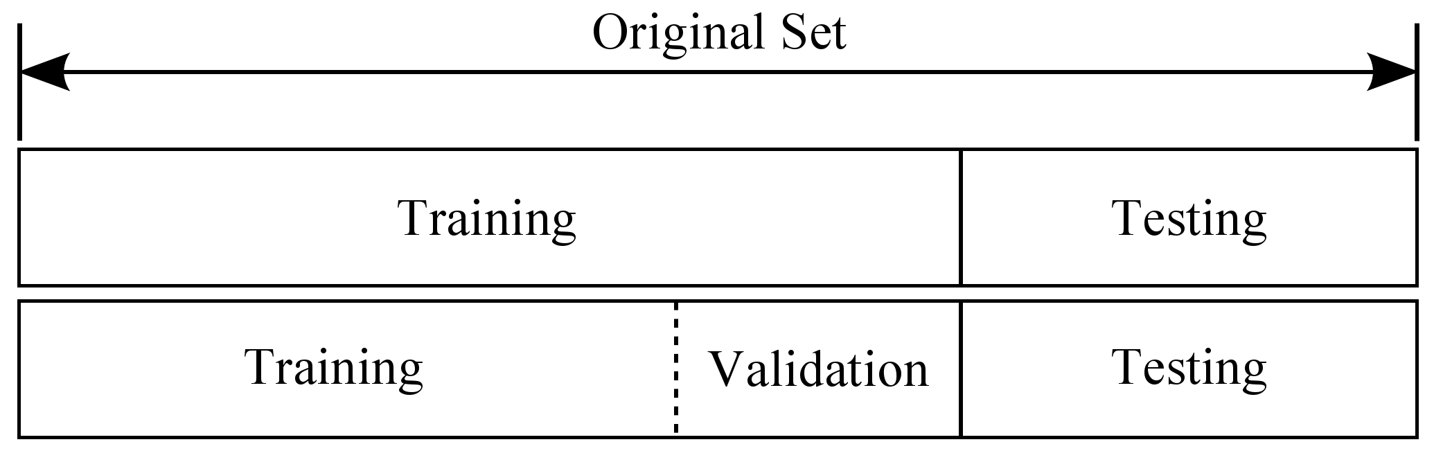
Source: https://rpubs.com/charlydethibault/348566
Divide a data set into three parts. Each part serves different purposes:
1. Use Training Data to estimate model parameters.
2. Use Validation Data to select model complexity.
3. Use Test Data to estimate Generalization Error.
Logistic Regression:
Draw a line between two classes of points.
Let there be two classes: $Y \in \{0,+1\}$
Logistic Function:
$g(x) = \dfrac{1}{1+e^{−w^T x}}$

Source: https://guide.freecodecamp.org/machine-learning/logistic-regression/
1. For points on a line: $w^Tx = 0$, and therefore $g(x) = 0.5$
2. For points on one side of a line: $w^Tx < 0$, and therefore $g(x) \rightarrow 0$
3. For points on one side of a line: $w^Tx > 0$, and therefore $g(x) \rightarrow 1$
1. Logistic Regression Model: A decision boundary $y = g(x) = \dfrac{1}{1+e^{−w^T x}} $ .
2. Learning: Estimate the model parameters $w$.
3. Cost Function: Cross Entropy
$ CE(w) = - \frac{1}{n} \sum_{i=1}^{n} \left\{ y_i \log g(x_i) + (1 − y_i) \log (1 - g(x_i)) \right\}$,
[ The gradient of the objective function is: $\nabla CE(w) = -\frac{1}{n} \sum_{i=1}^{n} (y_i - g(x_i)) x_i$ ]
4. Optimization Algorithm: Gradient Descent
Implementing Logistic Regression:
In [7]:
a1 = np.random.uniform(low=0, high=0.5, size=(100,2))
a2 = np.random.uniform(low=0.5, high=1, size=(100,2))
X = np.hstack((np.ones((200,1)), np.vstack((a1, a2))))
y = np.hstack(( np.zeros((100)), np.ones((100)) ))


def obj_fun(w):
    gx = 1 / (1 + np.exp(-np.dot(X, w)))
    # Implement Cross-Entropy
    return - np.mean((y * np.log(np.fmax(gx, 1e-9))) + ((1 - y) * np.log(np.fmax(1 - gx, 1e-9))))

def obj_grad(w):
    gx = 1 / (1 + np.exp(-np.dot(X, w)))
    # Implement the gradient of Cross-Entropy
    return - np.mean(np.reshape((y - gx), (X.shape[0],1)) * X, axis=0)


w0 = np.random.rand(X.shape[1]) * 2 - 1

res = minimize(fun=obj_fun, jac=obj_grad, x0=w0, method='CG')


print('Initial Guess =', w0)
print('Initial Obj Fun val =', obj_fun(w0))
plt.figure()
for i in range(2):
    plt.scatter(X[y==i,1], X[y==i,2], marker='x')
extreme_xvals = np.array([np.min(X[:,1]), np.max(X[:,1])])
plt.plot(extreme_xvals, (-w0[0] - w0[1] * extreme_xvals) / w0[2], c='r')
plt.show()
plt.figure()
for i in range(2):
    plt.scatter(X[y==i,1], X[y==i,2], marker='x')
final_w = res.x
print('Final w =', final_w)
print('Obj Fun val =', obj_fun(final_w))
plt.plot(extreme_xvals, (-final_w[0] - final_w[1] * extreme_xvals) / final_w[2], c='r')
plt.ylim(extreme_xvals+np.array([-0.05, 0.05]))
plt.show()


Application of Logistic Regression: Binary Classification of Handwritten '0's and '1's
In [9]:
from sklearn.datasets import load_digits
X, y = load_digits().data, load_digits().target
X = X[y<2,:]
y = y[y<2]
X = np.hstack((np.ones((X.shape[0],1)), X))
from sklearn.model_selection import train_test_split
X_train, X_test, y_train, y_test = train_test_split(X, y, test_size=0.1)


def obj_fun(w, X, y):
    gx = 1 / (1 + np.exp(-np.dot(X, w)))
    return -np.mean(y * np.log(np.fmax(gx, 1e-6)) + (1 - y) * np.log(np.fmax(1 - gx, 1e-6)))

def obj_grad(w, X, y):
    gx = 1 / (1 + np.exp(-np.dot(X, w)))
    return -np.mean(np.reshape(y - gx, (y.shape[0],1)) * X, axis=0)


min_cost = +np.inf
for i in range(10):
    w0 = (np.random.rand(X.shape[1]) * 2) - 1
    res = minimize(fun=obj_fun, jac=obj_grad, args=(X_train, y_train), x0=w0, method='CG')
    if res.fun < min_cost:
        min_w = res.x
        min_cost = res.fun


from sklearn.metrics import accuracy_score
print('Accuracy =',
      accuracy_score(y_test, np.round(1 / (1 + np.exp(-np.dot(X_test, min_w)))))
)
for i in range(5):
    plt.figure(dpi=50)
    plt.imshow(np.reshape(X_test[i,1:], (8,8)), cmap='gray')
    plt.xlabel(
        'Predicted Digit: '+str(int(np.round(1 / (1 + np.exp(-np.dot(X_test[i,:], min_w)))))),
    fontsize=24)
    plt.xticks([], [])
    plt.yticks([], [])
    plt.show()


